TOUGH4 User Manual
  • Quick Entry to Keywords for Data Input
  • 1️⃣INTRODUCTION
    • About TOUGH
    • TOUGH Development History
    • TOUGH4 Implementation
    • Scope and Methodology
  • 2️⃣WHAT IS NEW IN TOUGH4
  • 3️⃣CODE COMPILATION AND INSTALLATION
    • Setup for Compilation
    • Code Compilation
      • 1. Compilation of TOUGH4 using Visual Studio
      • 2. Compilation of TOUGH4 on Linux-like platform
    • Installation
    • Running the Executable for Simulations
  • 4️⃣GOVERNING EQUATIONS
    • Mass-Balance Equation
    • Accumulation Terms
    • Flux Terms
    • Sink and Source Terms
    • Virtual Node Well Treatment
    • Semi-Analytical Conductive Heat Exchange
    • Drift Model
    • Non-Darcy Flow
  • 5️⃣NUMERICAL METHOD
    • Space and Time Discretization
    • Interface Weighting Schemes
    • Initial and Boundary Conditions
      • Initial Conditions and Restarting
      • Neumann Boundary Conditions
      • Dirichlet Boundary Conditions
      • Atmospheric Boundary Conditions
      • Constant Temperature Boundary Conditions
    • Parallel computing schemes
    • Linear Solvers
    • Python Functions
      • Relative Permeability
      • Capillary Pressure
      • Initial Condition Calculation
      • Fetching Output Data
      • Fetching Thermophysical Property Data From NIST Webbook
      • Coupling With Third-Party Software
  • 6️⃣SOFTWARE ARCHITECTURE
    • Program Design
    • Data Structure
    • Linear Equation Setup
  • 7️⃣PROCESS MODELING
    • EOS1
    • EOS2
    • EOS3
    • EOS4
    • EOS6
    • EOS7
    • EOS9
    • ECO2
    • EWASG
    • TMVOC
    • Tracers/Decay Chain
    • Biodegradation Reaction
    • Wellbore Flow
    • Non-Darcy Flow
    • Enhanced Coal Bed Methane
  • 8️⃣PREPARATION OF MODEL INPUT
    • Input Formatting
    • Keywords and Input Data
      • TITLE
      • BIODG
      • CBMDA
      • CHEMP
      • COFT
      • CONNE
      • COUPL
      • DIFFU
      • ELEME
      • ENDCY
      • ENDFI
      • FLAC
      • FNIST
      • FOFT
      • FORCH
      • GASES
      • GENER
      • GOFT
      • HYSTE
      • INCON
      • INDOM
      • MESHM
      • MODDE
      • MOMOP
      • MULTI
      • OUTPU
      • PARAM
      • ROCKS
      • ROFT
      • RPCAP
      • SELEC
      • SOLVR
      • SPAVA
      • TIMBC
      • TIMES
      • TRACR
      • WELLB
    • Inputs for Initial Conditions
      • EOS1
      • EOS2
      • EOS3
      • EOS4
      • EOS6
      • EOS7
      • EOS9
      • ECO2
      • EWASG
      • TMVOC
    • Geometry Data
      • General Concepts
      • MESHMaker
      • Multiple-continuum processing
    • Inputs for MESHMaker
      • Generation of radially symmetric grids
        • RADII
        • EQUID
        • LOGAR
        • LAYER
      • Generation of rectilinear grids
      • MINC processing for fractured media
    • Adjustment of Computing Parameters at Run-time
  • 9️⃣OUTPUTS
  • 🔟VALIDATION AND APPLICATION EXAMPLES
    • EOS1
      • Problem 1 - Code Demonstration
      • Problem 2 - Heat Sweep in a Vertical Fracture (rvf)
      • Problem 3 - Five-spot Geothermal Production/Injection (rfp)
      • Problem 4 - Coupled Wellbore Flow (r1q)
      • Problem 5 - Five-Spot Geothermal Production/Injection under extremely high temperature
    • EOS2
      • Problem 1 -Five-spot Geothermal Production/Injection (rfp)
    • EOS3
      • Problem 1 - Code Demonstration (eos3p1)
      • Problem 2 - 1D TH Problem with Heating and Gas Source (by Guanlong Guo)
      • Problem 3 - Heat Pipe in Cylindrical Geometry (rhp)
      • Problem 4 - 3D Thermal Consolidation Test, Coupling with FLAC3D Simulator (by Guanlong Guo)
    • EOS4
      • Problem 1 - Code Demonstration (eos4p1)
      • Problem 2 - Heat Pipe in Cylindrical Geometry (rhp)
    • EOS6
      • Problem 1-Validation with EOS2
      • Problem 2-Noble Gas Transport
    • EOS7
      • Problem 1-Multiphase and Nonisothermal Processes in a System with Variable Salinity (rf1)
      • Problem 2-Thermal and Tracer Diffusion (EOS7R/rdif7)
      • Problem 3-Contamination of an Aquifer from VOC Vapors in the Vadose Zone (EOS7R/rdica)
      • Problem 4-Density, Viscosity, Solubility, and Enthalpy of Real Gas Mixtures (EOS7C/SAM7C1)
      • Problem 5-CO2 Injection into a Depleted Gas Reservoir (EOS7C2/SAM7C2)
      • Problem 6- CO2 Injection into a Saturated System (EOS7C/SAM7C3)
      • Problem 7-Density, Viscosity, and Enthalpy of Real Gas Mixtures (EOS7CA/SAM7CA1)
      • Problem 8-CO2 Injection into a Shallow Vadose Zone (EOS7CA/SAM7CA2)
      • Problem 9-Non-Isothermal Compressed Air Energy Storage in Reservoir (by Julien Mouli-Castillo)
    • EOS9
      • Page 1
    • ECO2
      • Problem 1-Demonstration of Initialization Options (ECO2N/rtab)
      • Problem 2-Radial Flow from a CO2 Injection Well (ECO2N/rcc3)
      • Problem 3-CO2 Discharge Along a Fault Zone (ECO2N/r1dv)
      • Problem 4-CO2 Injection into a 2-D Layered Brine Formation (ECO2N/rtp7)
      • Problem 5-Upflow of CO2 along a Deep Fault Zone (ECO2M/r1d)
      • Problem 6-Migration of a CO2 Plume in a Sloping Aquifer, Intersected by a Fault (ECO2M/rwaf)
      • Problem 7-GCS/GHE with a double-porosity reservoir (Case6_50kg_DP/ECO2NV2)
    • EWASG
      • Problem 1 - Brine Density Calculation (dnh)
      • Problem 2 - Production from a Geothermal Reservoir with Hypersaline Brine and CO2 (rhbc)
    • TMVOC
      • Problem 1-Initialization of Different Phase Conditions (r7c)
      • Problem 2-1-D Buckley-Leverett Flow (rblm)
      • Problem 3-Diffusion of components (rdif2)
      • Problem 4-Steam Displacement of a NAPL in a Laboratory Column (rtcem)
      • Problem 5-Steam Displacement of a Benzene-Toluene Mixture in a Laboratory Column (rbt)
      • Problem 6 -Air Displacement of a NAPL from a Laboratory Column (rad)
      • Problem 7-NAPL Spill in the Unsaturated Zone (r2dl)
    • T4.Well
      • Problem 1-Steady-state two-phase flow upward
      • Problem 2-Non-isothermal CO2 flow through a wellbore initially full of water
  • CONCLUSION REMARKS
  • REFERENCES
  • ACKNOWLEDGEMENT
  • Appendix
    • ☑️A: RELATIVE PERMEABILITY FUNCTIONS
      • IRP=1 Linear function
      • IRP=2 Power function
      • IRP=3 Corey's curves
      • IRP=4 Grant's curve
      • IRP=5 Perfectly mobile
      • IRP=6 Fatt and Klikoff function
      • IRP=7 van Genuchten-Mualem Model
      • IRP=8 Verma function
      • IRP=10 Modified Brooks-Corey Model
      • IRP=11 Modified van Genuchten Model
      • IRP=12 Regular hysteresis
      • IRP=13 Simple hysteresis
      • IRP=31 Three phase perfectly mobile
      • IRP=32 Modified Stone's first 3-phase method
      • IRP=33 Three-phase Parker's function
      • IRP=34 Alternative Stone 3-phase
      • IRP=35 Power-law function
      • IRP=36 Faust for two-phase Buckley-Leverett problem
      • IRP=37 Another alternative to Stone function
      • IRP=40 Table lookup
      • IRP=41 User-Defined relative permeability function
    • ☑️B: CAPILLARY PRESSURE FUNCTIONS
      • ICP=1 Linear function
      • ICP=2 Function of Pickens
      • ICP=3 TRUST capillary pressure
      • ICP=4 Milly’s function
      • ICP=6 Leverett’s function
      • ICP=7 van Genuchten function
      • ICP=8 No capillary pressure
      • ICP=10 Modified Brooks-Corey Model
      • ICP=11 Modified van Genuchten Model
      • ICP=12 Regular hysteresis
      • ICP=13 Simple hysteresis
      • ICP=31 Parker et al 3-phase function
      • ICP=32 Parker 3-phase function, alternative 1
      • ICP=33 Parker 3-phase function, alternative 2
      • ICP=34 Parker 3-phase function, alternative 3
      • ICP=40 Table lookup
      • ICP=41 User-Defined capillary pressure function
    • ☑️C: ADDITIONAL PROGRAM OPTIONS
    • ☑️D: DESCRIPTION OF FRACTURED FLOW
      • Multiple Continuum Approaches
      • Active Fracture Modle
Powered by GitBook
On this page
  1. PREPARATION OF MODEL INPUT
  2. Geometry Data

Multiple-continuum processing

PreviousMESHMakerNextInputs for MESHMaker

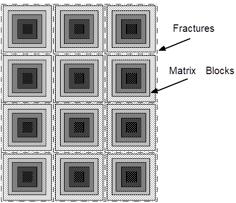
Multiple-continuum processing for simulation of flow in naturally fractured reservoirs can be invoked by means of a keyword MINC, which stands for “multiple interacting continua” (Pruess and Narasimhan, 1982, 1985). The MINC-process operates on the data of the primary (porous medium) mesh as provided on file MESH, and generates a “secondary” mesh containing fracture and matrix elements with identical data formats on file MINC. By appropriate subgridding of the matrix blocks, as shown in Figure 28, and therefore by resolving the driving pressure, temperature, and mass fraction gradients at the matrix and fracture interface, the transient, multiphase interporosity flows between rock matrix and fractures can accurately be described. The MINC concept is based on the notion that changes in fluid pressures, temperatures, phase compositions, etc. due to the presence of sinks and sources (production and injection wells) will propagate rapidly through the fracture system, while invading the tight matrix blocks only slowly. Therefore, changes in matrix conditions will (locally) be controlled by the distance from the fractures. Fluid and heat flow from the fractures into the matrix blocks, or from the matrix blocks into the fractures, can then be modeled by means of one-dimensional strings of nested grid blocks, as shown in Figure 28. The MINC-method lumps all fractions within a certain reservoir subdomain into continuum # 1, all matrix material within a certain distance from the fractures into continuum # 2, matrix material at larger distance into continuum # 3, and so on. Quantitatively, the subgridding is specified by means of a set of volume fractions, into which the primary porous medium grid blocks are partitioned. The MINC-process in the MESHMaker module operates on the element and connection data of a porous medium mesh to calculate, for given data on volume fractions, the volumes, interface areas, and nodal distances for a secondary fractured medium mesh. The information on fracturing (spacing, number of sets, shape of matrix blocks) required for this is provided by a “proximity function” PROX(x) which expresses, for a given reservoir domain Vo, the total fraction of matrix material within a distance x from the fractures. If only two continua are specified (one for fractures, one for matrix), the MINC approach reduces to the conventional double-porosity method (Warren and Root, 1963). Full details are given in a separate report (Pruess, 1983). For any given fractured reservoir flow problem, selection of the most appropriate gridding scheme must be based on a careful consideration of the physical and geometric conditions of flow. The MINC approach is not applicable to systems in which fracturing is so sparse that the fractures cannot be approximated as a continuum.

The file MESH used in this process can be either directly supplied by the user, or it can have been internally generated either from data in input blocks ELEME and CONNE, or from RZ2D or XYZ mesh- making. The MINC process of sub-partitioning porous medium grid blocks into fracture and matrix continua will only operate on active grid blocks, while inactive grid blocks are left unchanged as single porous medium blocks. In TOUGH4, elements in data block ELEME (or file MESH) are taken to be “active” unless they are specified as "inactive" or have very large volumes, which are taken to be “inactive.” In order to exclude selected reservoir domains from the MINC process and make them remain single porous media, the user needs to change the volume of the corresponding blocks to a very large number before MINC partitioning is made. Note that here the concept of inactive blocks is used in an unrelated manner with respect to the one to maintain time-independent .

8️⃣
Dirichlet boundary conditions
Figure 28 Subgridding in the method of "multiple interacting continua" (MINC).