EWASG

1. Description

The original EWASG (WAter-Salt-Gas) fluid property module was developed by Battistelli et al. (1997) for modeling geothermal reservoirs with saline fluids and non-condensible gas (NCG). In contrast to EOS7, EWASG describes aqueous fluid of variable salinity not as a mixture of water and brine, but as a mixture of water and NaCl. This makes it possible to represent temperature-dependent solubility constraints, and to properly describe precipitation and dissolution of salt.

In TOUGH4, EWASG extends to flow systems with components of water, multiple gases, multiple salts and optional heat as three-phase mixtures. The gas components can be any combination of 1-4 gases of the seven available gases (CH4, H2S, CO2, N2, O2, H2, and AIR). It allows including as many as 5 different salts. Solid salts are in an active mineral phase, which is treated in complete analogy to fluid phases (aqueous, gas), except that, being immobile, its relative permeability is identically zero. From mass balances on salts in fluid and solid phases we calculate the volume fraction of precipitated salts in the original pore space $\phi_0$, which is termed “solid saturation,” and denoted by $S_s$. A fraction $\phi_0 S_s$of reservoir volume is occupied by precipitate, while the remaining void space $\phi_f=\phi_0(1-S_s)$ is available for fluid phases. We refer to $\phi_f$as the “active flow porosity.” The reduction in pore space reduces the permeability of the medium (see below for the discussion of Permeability Change).

(1) Fluid thermophysical properties

Similar to the EOS7 module, the new EWASG also uses a cubic equation of state along with a multiphase Darcy’s Law to model flow and transport of gas and aqueous phase mixtures over a wide range of pressures and temperatures appropriate to typical subsurface gas/energy storage sites and natural gas reservoirs. The real gas properties module has options for Peng-Robinson, Redlich- Kwong, or Soave-Redlich-Kwong equations of state to calculate gas mixture density, enthalpy departure, and viscosity. Air is specially treated as a pseudo-component (AIR) with properties reflecting a mixture of two gas components, i.e., 79% N2 and 21% O2 (by volume), in solving the selected real gas cubic equation of state. Solubility of gases is calculated using a very accurate chemical equilibrium approach, the same approach as in EOS7. Transport of the gaseous and dissolved components is by advection and Fickian molecular diffusion. Details for the calculation of real gas properties and solubilities can be found on the EOS7description page. In TOUGH4/EWASG, gas solubility depends not only on temperature but also on salinity to describe the reduction in gas solubility with increasing salinity ("salting out"). The dependence of brine density, enthalpy, viscosity, and vapor pressure on salinity is taken into account, as are vapor pressure-lowering effects from suction pressures (capillary and vapor adsorption effects).

(2) Assumptions for salts

The current version of EWASG has a very simple solubility model for salts other than NaCl. It is assumed that all salts have the same solubility in water as NaCl. Their impacts on the gas solubilities and the thermophysical properties of aqueous phase are also assumed to be the same as NaCl. In addition, the mass fractions of the salts in solid phase are assumed equal to the corresponding mass fractions in aqueous phase. Improvement for handling the multiple salts may be needed.

(3) Permeability change

As noted above, the relationship between the amount of solid precipitation and the pore space available to the fluid phases is very simple. The impact of porosity change on formation permeability on the other hand is highly complex. Laboratory experiments have shown that modest reductions in porosity from chemical precipitation can cause large reductions in permeability (Vaughan, 1987). This is explained by the convergent-divergent nature of natural pore channels, where pore throats can become clogged by precipitation while disconnected void spaces remain in the pore bodies (Verma and Pruess, 1988). The permeability reduction effects depend not only on the overall reduction of porosity but on details of the pore space geometry and the distribution of precipitate within the pore space. These may be quite different for different porous media, which makes it difficult to achieve generally applicable, reliable predictions. EWASG offers several choices for the functional dependence of relative change in permeability, k/k0, on relative change in active flow porosity.

$\dfrac{k}{k_0}=f(\dfrac{\phi_f}{\phi} )\equiv f(1-S_s)$ (7-25)

The simplest model that can capture the converging-diverging nature of natural pore channels consists of alternating segments of capillary tubes with larger and smaller radii, respectively; see Figure 21. While in straight capillary tube models' permeability remains finite as long as porosity is non-zero, in models of tubes with different radii in series, permeability is reduced to zero at a finite porosity.

Figure 21. Model for converging-diverging pore channels

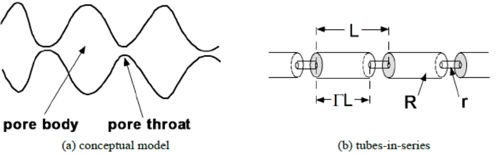
From the tubes-in-series model shown in Figure 1, the following relationship can be derived (Verma and Pruess, 1988)

$\dfrac{k}{k_0}=\theta ^2\ \dfrac{1-\Gamma+\Gamma/\omega^2}{1-\Gamma+\Gamma[\theta/(\theta+\omega-1)]^2}$ (7-26)

where

$\theta=\dfrac{1-S_s-\phi_r}{1-\phi_r}$ (7-27)

depends on the fraction 1- $S_s$ of original pore space that remains available to fluids, and on a parameter $\phi_r$, which denotes the fraction of original porosity at which permeability is reduced to zero. $\Gamma$ is the fractional length of the pore bodies, and the parameter $\omega$ is given by

$\omega=1+\dfrac{1/\Gamma}{1/\phi_r-1}$ (7-28)

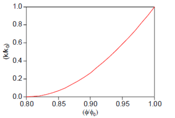
Therefore, Eq. (7-26) has only two independent geometric parameters that need to be specified, $\phi_r$ and $\Gamma$. As an example, Figure 22 shows the permeability reduction factor from Eq. (7-26), plotted against $\phi /\phi_0 \equiv (1-S_s)$ , for parameters of $\phi _r=\Gamma=0.8$.

Figure 22. Porosity-permeability relationship for tubes-in-series model after Verma and Pruess (1988)

For parallel-plate fracture segments of different aperture in series, a relationship similar to Eq. (7-26) is obtained, the only difference being that the exponent 2 is replaced everywhere by 3 (Verma and Pruess, 1988). If only straight capillary tubes of uniform radius are considered, we have $\phi _r=0$, $\Gamma=0$, and Eq. (7-26) simplifies to

$k/k_0=(1-S_s)^2$ (7-29)

1. Specifications

A summary of EWASG specifications is given in Table 14. The default number of mass components is 3 (water, one user selected gas and one salt). The maximum number of components is 10. The default choice of primary thermodynamic variables is (P, Xg, Xs, T) for single-phase, (Pg, Sg + 10, Xs, T) for two-phase conditions. The last primary variable is always temperature no matter if the simulation is in isothermal or non-isothermal, but in isothermal simulation the energy equation does not need to be solved and temperature is always constant. Xs is salt mass fraction if Xs<=1.0, is solid phase saturation plus 10 if Xs>=10.0. The component numbering is based on the number of gases and salts included in the simulation. For example, gas1 is always component 2, gas2 is component 3, gas3 is component4, and gas4 is component 5. If the model has 1 gas, 2 gases, 3 gases or 4 gases, the salt 1 will be component 3, 4, 5, 6 respectively. The component number of salts is the component number of last gas component plus the numbering of the salts.

Table 14 Summary for EWASG

Specification	Parameters
Components	(1) Water (2) Gases (at least 1 gas, at most 4 gases, gas 2-4 are optional) (3-7) Salt1-Salt5 (salt 2-5 are optional)
Phase condition and its state name and index $^*$	(1) Gas, GAS (2) Aqueous, AQU (3) two-phase, AQG
Primary variables	See Table 27
Optional process modeling	Molecular diffusion, Vapor pressure Lowering, Wellbore simulation, Biodegradation reactions, and non-isothermal simulation.

$*$ Solid salts can exist in any of the three phase conditions

1. Specific input requirements

Various options for EWASG can be selected through parameter specifications in data block SELEC, as follows.

IE(3) allows choice of brine viscosity calculation.

0: after Phillips et al. (1981) (default).

1: after Palliser and McKibbin (1998).

2: after Mao and Sun (2006).

3: after Potter (1978).

IE(4) allows choice of correlation for compressed brine density.

1: after Andersen et al. (1992) (default = 0).

2: Pritchett (1993).

3: Brine compressibility equal to water compressibility at the same reduced temperature.

4: Brine compressibility equal to water compressibility at the same temperature.

5: after Batzle and Wang (1992).

6: after Driesner (2007) .

IE(10)/IE(24) allows to turn vapor pressure lowering on/off (IE(10) is for EWASG only).

0: VPL is off.

1: VPL is on.

IE(11) selects dependence of permeability on the fraction $\phi_f /\phi_0=(1-S_s)$ of original pore space that remains available to fluids.

0: permeability does not vary with $\phi_f$.

1: $k/k_0=(1-S_s)^\gamma$, with $\gamma=FE(1)$.

2: fractures in series, i.e., Eq. (7-26) user manual with exponent 2 everywhere replaced by 3.

3: tubes-in-series, i.e., Eq. (7-26) .

IE(13) allows choice of dependence of brine density on dissolved CO2.

0: brine density varies with dissolved CO2-concentration, according to García's (2001) correlation (Eqs. 13-14) for temperature dependence of molar volume of dissolved CO2.

1: brine density is independent of CO2 concentration.

IE(14) allows choice of treatment of thermophysical properties as a function of salinity.

0: full dependence.

1: no salinity dependence of thermophysical properties (except for brine enthalpy; salt solubility constraints are maintained).

2: no salinity dependence of thermophysical properties including brine enthalpy

IE(15) allows choice of correlation for brine enthalpy at saturated vapor pressure

0: after Lorenz et al. (2000).

1: after Michaelides (1981).

2: after Miller (1978).

3: after Phillips et al. (1981).

4: after Lorenz et al. (2000) (default = 0).

5: after Driesner (2007).

IE(18) turn on/off the impact of permeability change caused by solid precipitation /dissolution in flux calculation

0: off

1: on, the changed permeability will be used for calculation of flux between two grids.

IE(23) Set equal to 0 to use ZEVSREAL for enthalpy of gas mixture, Set equal to 1 to use SUPST for water vapor, and ZEVSREAL for other gases, with a weighted sum used for the mixture enthalpy.

FE(1) parameter γ (for IE(11)=1); or parameter $\phi_r$(for IE(11) = 2, 3)

FE(2) parameter $\Gamma$ (for IE(11) = 2, 3)

EWASG requires definition for gases and salts which are included in the simulation. The inputs for gas definition are by keyword "GASES", and salt definition borrows the definition of tracer by keyword "SALTS" or "TRACR".